“Education for the Masses?:
The Interaction between Wealth, Educational and Political Inequalities”

Francisco H.G. Ferreira

Keywords: Inequality, Education, Political Economy
JEL Classification Numbers: D31, D63

Abstract: This paper presents a simple model of distribution dynamics in which non-convexities in the private education production function and politically determined fiscal redistribution in kind combine to generate Pareto and Lorenz rankable equilibria. Agents choose between low-quality free public schools and high-quality fee-paying private schools. The quality of public education is determined endogenously, through voting on its financing. Voting power may vary with wealth. For some levels of public spending, the poorest agents are prevented from attending their first-best choice of school by a missing credit market. Under these conditions, it is shown that the multiple equilibria which are possible include a Pareto-inferior, high-inequality equilibrium. In this equilibrium, wealth, educational and political inequalities mutually reinforce one another. Escaping this high-inequality trap, which could lead to a welfare dominant allocation, may require a change in the distribution of voting power.

“To the extent that the probability of children earning increased income in the future is influenced by parents’ income, equality of opportunity will not prevail, and inequality will tend to persist.”
- Albert Fishlow, 1972, p.392.

1. Introduction.

The persistence of wealth or income inequality in the long-run is an empirical regularity worthy of mention alongside Nicholas Kaldor’s (1963) six stylized facts of economic growth. A considerable body of both theoretical and empirical literature has recently proposed and tested a variety of mechanisms through which inequality may not only persist among agents with equal preferences and initial skill endowments, but also lead to inefficient aggregate outcomes in steady-state.

At the risk of oversimplifying, these mechanisms can be grouped under two broad categories. The first relies on imperfect capital markets and non-convex production sets, which combine to prevent a group of agents (usually but not always the poor) from exercising their full economic potential. The second relies on political economy channels, through which greater inequality may either lead to more inefficient redistribution (Alesina and Rodrik, 1994; Persson and Tabelini, 1994) and thus lower growth rates, or to greater political instability and social conflict (e.g. Rodrik, 1997). More recently, the two strands have promisingly combined, as researchers seek to capture the interplay between the political determinants of (redistribution) policies, and the effect of information asymmetries and incomplete contracts on differentiated access to credit and insurance markets along the wealth distribution. In particular, Bénabou (2000) shows that risk-averse agents in a stochastic environment with incomplete insurance markets will derive positive utility from redistribution as an imperfect, publicly provided substitute for insurance. The combination of efficient (i.e. welfare-increasing) redistribution and unequally distributed political power generate the possibility of multiple political-economic equilibria, where the most equal is characterized by the highest degree of redistribution, and the most unequal has the least redistribution. This result is at odds with the predictions of some of the earlier political economy models of the dynamics of income distribution (e.g. Alesina and Rodrik, 1994 and Persson and Tabellini, 1994), and conforms better with the empirical evidence found by Perotti (1996) and others.

Bénabou (2000) also considers the financing of public education in an extension of the model. The market for education loans is missing, and tax revenues are redistributed as education subsidies (effectively through demand-side vouchers). The nature of the equilibria remains unchanged from his main model: although the high inequality equilibrium displays less redistribution, the two equilibria are not Pareto-rankable. This result depends on specific assumptions, such as the convexity of the education production set and the lognormality of the p.d.f.s of the random shocks.

This paper shows that stronger equity-efficiency relationships can obtain if we allow for the existence of education non-convexities, and if the government is able to make in-kind, rather than cash transfers. The model combines a voting mechanism, through which policies are determined endogenously, with an imperfect credit market, to shed light on a vicious circle of interaction between educational, wealth and political inequalities, which may lead to the existence of inefficient high-inequality equilibria. If educational opportunities differ for people along the wealth distribution, and the quality of the education available to the poor depends on an endogenously determined redistribution scheme (such as funding public schools from general proportional taxation), then a distribution of power that mirrors an unequal distribution of income may lead to persistent and inefficient levels of inequality.

The focus on the nature of redistribution through public education is shared with a number of recent papers, such as Bénabou (1996) or Fernandez and Rogerson (1995, 1998). Unlike these, however, I am less concerned with the degree of centralization of the public financing of education, and more with its quality relative to that of its private alternatives, and the effect this has on effort levels, the distribution of human capital, aggregate productivity, and the distributions of income and political power. Unlike Fernandez and Rogerson (1995), assumptions about the inferior quality of public education are made which are more compatible with primary and secondary schooling in a country like Brazil or the United States, rather than with higher education in the same countries. Although the basic problem is similar to that studied by Glomm and Ravikumar (1992), our results are quite different, largely because we do not assume that human capital bequests (as opposed to physical ones) exist and that these are taken into account by agents in a private-education economy but not by those in a public-education one.

2. The Model

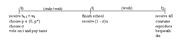
Let there be a continuum of agents with initial wealth levels w distributed over (0, z), according to G(w). These agents consist of households which are ex-ante identical in every respect, except their initial wealth. Their size is normalised to one, and no intra-household issues are considered. Household labour supply is inelastic, and I assume that the nature of available projects is such that labour can not be pooled across households. Generations are successive and do not overlap. Their finite lives have two periods, according to the linear sequence below:

Figure 1:



 

---

These agents maximise a utility function based on Andreoni’s (1989) “warm glow” bequest motive:

         (1)

where, as denoted in figure 1, both consumption and bequeathing take place at life’s end, time t₂. Consumption and bequest are of a single consumption good, which is chosen as the numeraire good. This good is produced by skilled and unskilled workers, whose productivity levels and remuneration rates differ, but each unit of the good emerging from both processes is identical. It is costlessly storable and does not depreciate over time.

In the first period, they allocate their time fully between two activities: studying or working as an unskilled worker, whose deterministic productivity (and remuneration rate) is u. At time t₀ they choose s (0 < s < 1): the fraction of time in the first period spent studying. Studying can take place through either one of two mutually exclusive education technologies. These are distinguished by different prices and productivity levels, but produce the same good: embodied human capital S, an excludable and non-transferable attribute of each individual student. The price of enrolling in the education production function 1, which we will associate with private schooling, is p₁ = p* > 0. The price of enrolling in the education production function 2, which we will associate with public schooling, is p₂ = 0. The choice of school type, which is distinct from the time allocation decision, is denoted in Figure 1 as a choice of p. The choice is made under the knowledge that:

         if p = p* and         (2a)

     if p = 0.             (2b)

 

The education productivity parameter q > 0 converts time spent in school into actual human capital. I assume that (Assumption 1), where p is defined immediately below. t is total public spending on education.

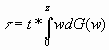
In the second period, agents dedicate their full time endowment to skilled work. Each agent’s productivity (and remuneration) is assumed to be an increasing linear function of their acquired level of human capital: p S. Since agents pay tax on their inheritance at time t₀, final income available at t₂ for consumption and bequests is given by:

     (3)

Credit markets are assumed to be completely absent in this economy, as a result of extreme problems in enforcing contracts.

The political system functions as follows. Lump sum taxes and transfers are administratively unfeasible and the constitution mandates that all taxation be in the form of proportional wealth taxation at the beginning of each generation’s life. All public expenditures must be directed towards financing public education, through t . Budget balance at every generation is also constitutionally mandated so that . Individually preferred tax rates are monotonically declining with wealth, so that the single tax rate t* is chosen by the critical voter:

(4)

where the wealth of critical voter is w_c and the critical voter is such that:

     (5)

v(w) is the voting power function, which is assumed here to depend (weakly) positively on the individual’s initial wealth level. V(w) may take many forms, provided it satisfies: v’(w) ł 0 and 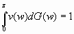. Two examples of voting power functions which satisfy these two properties and have plausible empirical interpretations are:

(i) v(w) = 1 Ž      “one person, one vote” or democracy

(ii) Ž     “money talks” or oligarchy.

 

3. The Static Equilibrium.

There are three control variables in the model: c (or b), p and s . At time t₀ agents choose p and s . Through voting, the critical agent chooses t*, which can be taken as given by all other agents. The consumption/bequest allocation of final income is decided at time t₂ and is independent of the remaining choices.

Lemma 1: Given Assumption 1, p = 0 for any agent with wealth w < p*(1-t*)^-1, and p = p* for any agent with wealth w ł p*(1-t*)^-1.
Proof: See appendix.

This means that the quality (or productivity) differential between private and public schools is so large, that any agent capable of affording private education will choose to do so. Since credit markets have been assumed away, these are only those agents whose initial wealth level net of taxes at least equals the (exogenously given) private school fee.

Lemma 1 partitions each generation at the outset, into those which will attend private school (using education technology 2^a) and those which will attend public school (using technology 2b). In conjunction with the fixed good-production productivity parameters u and p , this knowledge of the education technology at their disposal allows each agent to determine an optimal first-period time allocation.

 

For agents with w < p*(1-t*)^-1, the problem is to , which is obtained by substituting (2b) into (3). The first order condition implies that:

(6)

 

Similarly, for agents with w ł p*(1-t*)^-1, the problem is to , which is obtained by substituting (2a) into (3). The first order condition implies that:

         (7)

 

Once t* is determined through the t₀ voting process, and agents have chosen p and s , we can complete a full characterisation of the static equilibrium by describing the final incomes accruing to each agent. Replacing the appropriate values p(w) - from Lemma 1 - and s (w) – from (6) or (7) - into equation (3), the total income function is as follows:

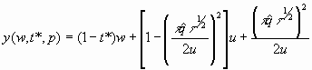if w < p*(1-t*)^-1, (8a)

 

if w ł p*(1-t*)^-1. (8b)

 

Considering t* (and thus t ) as given for each agent, the second and third terms on the right hand side of (8a), as well as the second, third and fourth terms on the right hand side of (8b) consist solely of exogenous parameters. Let the sum of those terms in (8a) be denoted by A and the sum of those terms in (8b) be denoted by B. These equations can then be rewritten in short form as:

 

         if w < p*(1-t*)^-1,         (9a)

         if w ł p*(1-t*)^-1,         (9b)

 

Note that A < B, from Lemma 1 (see proof in the appendix). This implies that incomes are monotonically rising in initial wealth (with derivative less than one), but with a discontinuity at the wealth level which allows agents to attend the superior private schooling system.

Finally, it is worth noting the following comparative properties of the time allocation choices across the two different groups of agents, from equations (6) and (7). For both private and public school students, and , as one would expect. The first inequality shows that effort spent in human capital accumulation declines with its opportunity cost, the remuneration for unskilled work. The second inequality shows that the effort (or time) allocation for human capital accumulation increases with its expected benefit, the rate of remuneration of skilled labour.

 

More interestingly, however, note that , implying that public expenditures on schooling raise the time (or effort) spent by students in acquiring human capital. The impact of higher public education spending is therefore twofold: there is a direct productivity impact, which raises the output S for a given level of agent effort, through equation 2b. This impact is positive but concave, so that decreasing returns to this kind of spending hold. There is also, however, an indirect impact through the behavioural response of agents to higher school quality. This is nothing but an application of the Keynes-Ramsey rule: as the marginal rate of transformation (of current time into future human capital) rises, the marginal rate of intertemporal substitution (between current and future income) must rise accordingly at the optimum. Since a higher t makes time spent studying more productive, agents respond by allocating more such time, and giving up a little more first period income.

Finally, for levels of t consistent with Assumption 1 (which places an upper bound on t , given the educational productivity parameters), . This means that in societies where the gap between the ‘quality’ of private education () and that of public education systems () is sufficiently large with respect to the price of private education (p*) – see Assumption 1 – one will observe the poorest people in society attending worse schools and dedicating less time (or effort) to their studies. In this model, this arises from optimising behaviour in the face of missing credit markets and exogenous ‘quality’ differences, despite identical preferences across agents. An observationally equivalent outcome (of less dedicated students of public schools being the poorest) might be generated from a very different model, in which there were no missing markets (i.e. opportunities did not depend on initial wealth), but some people were lazier or less intelligent than others. The implication is that before judging which of the two models is correct – whether the poor study less as an optimal response to unequal opportunities or whether they are poor because they are lazy people living in a fair system – one would have to test the two models with respect to other predictions, or directly with respect to whether their assumptions hold in practice.

4. Transitional Dynamics and the Multiple Steady-States

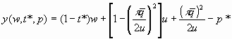
Maximisation of the Andreoni “warm glow” utility function in (1) implies that each agent sets c = a y(w, t*, p) and b = (1- a ) y(w, t*, p) at time t₂ , where the final income function is given by equations (8) or (9). Since bequests constitute the only link between generations in the model, the law of motion of the state variable wealth is fully characterised by equation (10) below:

         if w_t < p*(1-t*)^-1,         (10a)

             if w_t ł p*(1-t*)^-1,                (10b)

 

Again, because the political equilibrium depends only on contemporaneous variables, and does not establish a separate link between generations, and because the other parameters in A and B are exogenous and constant, equation (10) depicts a unidimensional Markov process. For a given set of exogenous parameter values, this dynamic process will converge to a unique invariant limiting distribution.

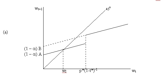
Figure 2 below shows three examples of such transition processes (and their limiting distributions), for different parameter values. The three panels of Figure 2 plot the intergenerational transition function (10) for different values of the intercepts A and B, which reflect different underlying values for the unskilled and skilled productivity parameters (u and p ), and/or for the educational production function parameters (). Since there is no stochastic term in the model, any initial distribution defined over (0, z) – or indeed  *₊ - will converge to the attractor wealth levels where w_t+1 = w_t. This implies three broad classes of equilibria for this model. The first, depicted diagrammatically in panel (a), sees a disappearance of the privately educated class. Returns to schooling relative to its private market price are insufficient to sustain bequests capable of preventing this inexorable downward mobility. Equilibrium will be characterised by perfect wealth equality, and universal public education.

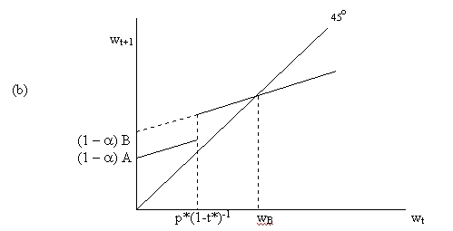
The second type of steady-state, depicted in panel (b), is also marked by complete wealth equality, but with education being provided solely by the private market. Returns to schooling, relative to its private market price, are high enough that everyone eventually acquires sufficient education and makes sufficiently large bequests so that no one is left with inheritances below the cut-off wealth value p*(1-t*)^-1.

Figure 2:







 

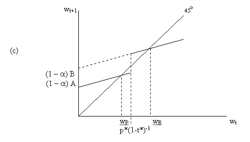
The third type of equilibrium is the one on which I wish to focus. Here, there are two unequal wealth classes. Any lineage whose initial wealth level is below the critical value p*(1-t*)^-1 will converge towards a ’poor’ attractor at w_P . Those lineages fortunate enough to start off with levels of wealth above the threshold converge instead to a ‘rich’ attractor at w_R. The ‘poor’ can not afford private schooling, even though this would make them more productive. The absence of credit markets prevent them from exploiting that possibility. All the ‘rich’ choose private schooling. Bequests are such that once this situation is reached, it is a stable equilibrium. Unless it is perturbed – say, by a change in the political equilibrium that determines public spending on education – such a society would remain thus economically and educationally divided forever.

5. Political Equilibria

The one variable as yet undetermined, and which has an effect on the incomes of publicly educated agents (through the intercept term A in Figure 2), is the level of public spending t or, equivalently, the tax rate t*. Assumption 1, which determined the constellation of parameter values within which the model would be investigated, aimed to exclude high values of t* (relative to p*), so that y(w, t*, p*) > y(w, t*, 0), " w. If it were relaxed, it would clearly be possible to set t at an arbitrarily high level, so that A = B, and agents were indifferent between public or private education at every wealth level. Or indeed, to drive private education out of the model ex-ante (rather than in equilibrium, as in panel (a)), by having A > B.

Our concern, however, is not with governments that can set arbitrary values of t . Instead, as set out in Section 2, we have in mind a political economy equilibrium where a critical agent (in terms of voting power) takes a decision about t, based on her own selfish interests. If we now restrict our attention to the stable unequal equilibrium depicted in panel (c) of Figure 2, it is clear that if w_c > p*(1-t*)^-1 , t* = 0, since those agents do not benefit from public expenditure at all.

A non-zero value of t* will in general be obtained from

         (4’)

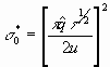
for w_c < p*(1-t*)^-1 . Setting , and noting that implies that , we find that . This preferred tax rate is duly monotonically declining in personal wealth for all w < p*(1-t*)^-1, as claimed earlier. It goes to zero for w ł p*(1-t*)^-1.

Note that whenever the solution to this problem is consistent with the high-inequality equilibrium depicted in panel (c) above, it will be Pareto inefficient. This is because the maximisation of (4’) trades off marginal costs of the initial wealth taxation against the marginal gains from higher second-period income as a result of better schooling, but ignores the possibility of a discrete jump in equilibrium if D A(D t ) is sufficient to move the economy from a (c)-type equilibrium to a (b)-type equilibrium, as could clearly happen. This kind of discrete regime change would be characterised by a large increase in taxation and public expenditure on public education, followed by a transitional period of expansion in average educational attainment and rising incomes, which would eventually see a transition away from public and towards private schooling. This would be accompanied by falling wealth and educational inequality, and eventually falling tax rates. At the new steady-state, all agents in every generation would start off with the wealth level previously enjoyed only by the rich, but voting will ensure a zero tax rate which will make everyone better off.

But how could such a regime change be brought about, if a (c)-type equilibrium is stable? Such an economic and educational regime change may come about as a result of a change in the political power function v(w). Consider, for instance, a case in which equilibrium (c) holds, generating a wealth Lorenz curve L(w) of the general shape given by the kinked line in Figure 3 below:



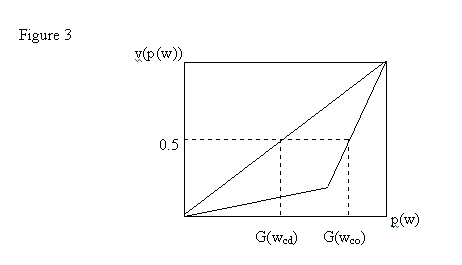
Suppose that initially . In this case, the critical agent has rank G(w_co), where o stands for “oligarchy”. Since preferences for t* decline monotonically with w, this outcome will yield a lower level of public expenditure t _o than that which would arise if v(w) = 1. In that case, the critical agent is poorer, with wealth level w_cd and rank G(w_cd). t* and t rise as a result. Although the magnitude of the increase depends on the specific closed-form solution, it is clear that a constellation of parameter values {u, p , p*, }exists such that an increase in t* of this nature will result in a change of regime from the inefficient, high-inequality (c)-type equilibrium to the more efficient and egalitarian (b)-type equilibrium.

6. Conclusions.

This paper presents a simple model of the joint determination of the distributions of education, wealth and power, in a setting where publicly provided education is of inferior quality than its privately provided substitute. Educational inequality may persist in steady state if (i) a missing credit market prevents the poorest agents to attend the better schools, reducing their lifetime wealth; and (ii) the voting equilibrium fails to generate sufficiently high public expenditure to increase the quality of the public schools attended by the poor.

If voting power is not distributed uniformly, but increases with private wealth, a self-sustaining high-inequality trap may arise, whereby educational inequality ensures the persistence of wealth inequality, which in turn ensures the persistence of political inequality, which in turn guarantees the continuation of educational inequality.

Such an equilibrium is inefficient in the sense that an alternative equilibrium with higher total wealth is attainable, through a temporary increase in taxes and public expenditures, so as to lift the poor out of the low education – low productivity trap. During the transition, this change is not Pareto improving, since higher taxes make the richer agents worse off. The new steady-state however, would Pareto dominate, first-order stochastically dominate and Lorenz dominate the former. If tax-and-spend decisions are fully endogenous, the only way to escape the initial, Pareto-dominated equilibrium is through a political regime change, which transfers political power from richer to poorer agents.

1. p Î {0, p*}. An agent with wealth level w will choose p* over 0 iff y(w, t*, p*) > y(w, t*, 0). That is, iff:

which is Assumption 1. This assumption thus sets an upper bound on t , given the values of p*, , u and p , such that Lemma 1 holds for any w.

2. Under this assumption, p = p* is preferred to p = 0, for any w. But since p* > 0 and there are no credit markets, p must be paid entirely out of initial after-tax wealth (1 – t*)w. It follows that only agents with can afford to effectively exercise their choice of p = p*. Agents with are constrained to choose p = 0.

References.

Aghion, Philippe and Patrick Bolton (1997): "A Trickle-Down theory of Growth and Development with Debt Overhang", Review of Economic Studies, 64 (2), pp. 151-172.

Alesina, A. and D. Rodrik (1994): “Distributive Politics and Economic Growth”, Quarterly Journal of Economics, CIX, 2, pp.465-490.

Andreoni, J. (1989): “Giving with Impure Altruism: applications to charity and Ricardian equivalence”, Journal of Political Economy, 97, pp.1447-1458.

Banerjee, A.V. and A.F. Newman (1991): "Risk Bearing and the Theory of Income Distribution", Review of Economic Studies, 58, pp.211-235.

Banerjee, A.V. and A.F. Newman (1993): “Occupational Choice and the Process of Development”, Journal of Political Economy, 101, No.2, pp.274-298.

Bénabou, Roland (2000): "Unequal Societies: Income Distribution and the Social Contract", American Economic Review, 90 (1), pp. 96-129.

Besley, Timothy and Stephen Coate (1991): "Public Provision of Private Goods and the Redistribution of Income", American Economic Review, 81, pp.979-984.

Fernandez, Raquel and Richard Rogerson (1995): "On the Political Economy of Education Subsidies", Review of Economic Studies, 62, pp. 249-262.

Fernandez, Raquel and Richard Rogerson (1998): "Public Education and Income Distribution: A Dynamic Quantitative Evaluation of Education-Finance Reform", American Economic Review, 88 (4), pp.813-833.

Ferreira, Francisco (1995): "Roads to Equality: Wealth Distribution Dynamics with Public-Private Capital Complementarity", LSE-STICERD Discussion Paper TE/95/286.

Fishlow, A. (1972): “Brazilian Size Distribution of Income”, American Economic Association: Papers and Proceedings 1972, pp.391-402.

Galor, O. and J. Zeira (1993): “Income Distribution and Macroeconomics”, Review of Economic Studies, 60, pp. 35-52.

Gans, Joshua and Michael Smart (1996), "Majority Voting with Single-Crossing Preferences", Journal of Public Economics, 59 (2), pp.219-237.

Glomm, Gerhard and B. Ravikumar (1992): "Public versus Private Investment in Human Capital: Endogenous Growth and Income Inequality", Journal of Political Economy, 100 (4), pp. 818-834.

Paes de Barros, R, M. Foguel, R. Henriques e R. Mendonça (1999): “O Combate ŕ Pobreza no Brasil: dilemas entre políticas de crescimento e políticas de reduçăo da desigualdade”, mimeo, IPEA (Rio de Janeiro).

Perotti, Roberto (1996): "Growth, Income Distribution and Democracy: What the Data Say", Journal of Economic Growth, 1 (2), pp.149-187.

Persson, T. and G. Tabellini (1994): “Is Inequality Harmful for Growth?”, American Economic Review, 84, 3, pp. 600-621.

Piketty, T. (1997): “The Dynamics of the Wealth Distribution and the Interest Rate with Credit Rationing”, Review of Economic Studies, 64, pp.173-189.

Rodrik, D. (1997): “ Where Did All the Growth Go?: External Shocks, Social Conflict, and Growth Collapses”, mimeo, Kennedy School, Harvard University (Cambridge, MA).

Stokey, Nancy and Robert Lucas (1989): Recursive Methods in Economic Dynamics (Cambridge, MA: Harvard University Press).

1) Department of Economics, Catholic University of Rio de Janeiro. I am grateful to Maurício Bugarin, Raquel Fernandez, Ricardo Paes de Barros and seminar participants at the London School of Economics, the Catholic University of Rio de Janeiro, the Getúlio Vargas Foundation at Rio de Janeiro, and the University of Brasília for helpful comments. All remaining errors are mine.
2) My translation.
3) For an example where the richest are constrained by the absence of a full insurance market, see Banerjee and Newman, 1991.
4) The list is now great, but seminal papers were written by Galor and Zeira (1993), Banerjee and Newman (1993), Aghion and Bolton (1997) and Piketty (1997).
5) Along the lines discussed by Besley and Coate (1991), but in a different dynamic context.
6) Human capital S is the only form of capital in this economy.
7) This initial wealth taxation can be interpreted as an ex-post inheritance tax. Very little changes if the tax is collected on final incomes at t₂ instead, but it is then harder to reconcile positive taxation with the utility function in (1).
8) See Section 5 for a proof. This result allows us to rely on the version of the median voter theorem implicit in (4), as established by Roberts (1977). See also Gans and Smart (1998).
9) Although (1) is written in terms of consumption and bequests, the Cobb-Douglas functional form implies that final income will be shared proportionately between the two uses, and every prior decision can be seen as taken to maximise end-of-period income.
10) Which in the case of this simple, deterministic system, is intuitive, but see Ferreira (1995) or Stokey and Lucas (1989) for increasingly more general proofs of the Markov convergence theorem.
11) See the proof of Lemma 1 in Appendix 1.
12) The subscript d stands for “democracy”.
13) That such a constellation exists can be seen intuitively from the fact that these parameter values can be chosen to make A and B arbitrarily close.